Genomics 3 - Workshop 4: RNAseq

Welcome to Workshop 4! This workshop will build on some of the skills you developed in previous courses using gene expression data. In previous courses you have worked with count data to look at gene expression, and to explore genes which are differentially expressed between conditions (such as in health and disease). This data has already been processed from raw reads: performing quality control, aligning to a reference genome or transcriptome, and then summarising to gene level. In this workshop you will do the whole process, from raw reads to differential expression analysis.
If you choose to base your final report on this workshop, you will need to use the hypoxia exposed urothelium dataset and not the BKPyV dataset used in this workshop . The bioinformatic approach will be very similar, but you will need to bring in relevant biology. More details on this dataset are at the end of the workshop material.

As ever, the workshop is aimed towards those with Windows machines, including the managed university machines. If you are using your own machine, you have a little more freedom. If you have a Mac, you should be aware of the differences by now (Terminal rather than PowerShell, etc.).

Before you get stuck in

As part of this workshop you will use the teaching0.york.ac.uk server, like last time. You will use linux modules and command line R. This should feel nice and familiar! This session will generate plots at the command line which you can then download. If you do RNAseq for your final report, you may want to take your final data off the server and explore with RStudio - this is absolutely fine! Always remember there are lots of different ways to compete the same task when you're coding.
As soon as you can, get logged on to the server and get the following R libraries installed. You will only need to do this once.

Open Windows PowerShell and log on to the server as before:

ssh USERID@teaching0.york.ac.uk

First, create a new shortcut to help with very long path names:

ln -s /shared/biology/bioldata1/bl-00087h/ genomics

# this means when you log in you can now do this to get to the genomics space
cd ~/genomics/

# you can also use ~/genomics in paths, rather than /shared/biology/bioldatat1/bl-00087h/
# I will use this throughout the workshop material

Change directory into your user space within the ~/genomics/students/ area, and make a new directory for this workshop, for example: workshop4. Change into that new directory. We are now ready to set up your R space.

# create directories for your newly installed R libraries to go (this helps with version control and installing on a managed machine)
mkdir ~/Rlibs ~/Rlibs/R_4.1.2

# type R to launch R from the linux terminal
R 

Within R, you can run the following lines one by one, or copy and paste in one go. If any package installations ask for updates, you can skip. Whilst these are installing, read the introductory material for the workshop below.

install.packages("ggrepel", lib="~/Rlibs/R_4.1.2")
install.packages("BiocManager", lib="~/Rlibs/R_4.1.2")
library("BiocManager", lib.loc="~/Rlibs/R_4.1.2")

BiocManager::install("tximport", lib="~/Rlibs/R_4.1.2")
BiocManager::install("rhdf5", lib="~/Rlibs/R_4.1.2")

install.packages("remotes", lib="~/Rlibs/R_4.1.2")
library("remotes", lib.loc="~/Rlibs/R_4.1.2")
remotes::install_github("pachterlab/sleuth", lib="~/Rlibs/R_4.1.2")
remotes::install_github("kevinblighe/EnhancedVolcano", lib="~/Rlibs/R_4.1.2")
remotes::install_github("ctlab/fgsea", lib="~/Rlibs/R_4.1.2")

q()

The q() command exits R and brings you back ready for the workshop.

Introduction to the material and research question in this workshop

Bladder cancer is the 10th most common global cancer and is one of the most expensive to treat as most cancers recur and when the disease progresses, standard practice is to remove the bladder. Despite such radical surgery, 5-year survival is <50% in muscle-invasive disease.
There is therefore an unmet need to understand how bladder cancers start, and what can be done to prevent them. The long-standing risk factor for bladder cancer is smoking, but mutational signatures (see lecture 7 if you're unsure what these are) showed that the classic mutational profile of smoking seen in lung cancer is not present in bladder cancer. Instead, there are signatures of APOBEC mutagenesis - a family of enzymes which defend against viruses. These signatures are very prevalent in HPV-driven cervical cancers. However, there is no obvious viral cause for bladder cancer, and viral genomes are not found within bladder cancer genomes (as they are with HPV positive cervical cancer).

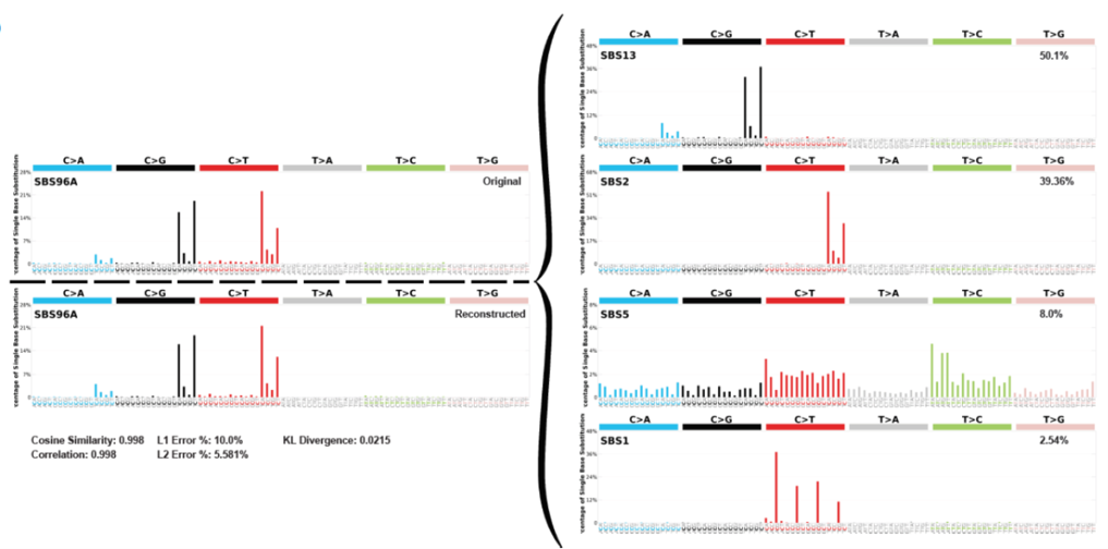
Deconvolution of mutational signatures. Top left plot shows the original proportion of single base substitutions in the sample. The right hand side shows the deconvolution into separate SBS derivations and their relevant proportions, and as proof the bottom left plot shows the reconstruction of the signature using the deconvoluted plots.

Based on epidemiolgical data, and high incidence of bladder cancer in kidney transplant patients, researchers at York hypothesised that BK Polyomavirus (BKPyV) may be the cause. The RNAseq data in this workshop was our first effort to explore this association and formed part of a publication in Oncogene in 2022.

The workshop

Hopefully your R libraries have finished installing, if not it hopefully won't be too much longer.
All the workshop material is in:

~/genomics/rnaseq_data/01_workshop4_BKPyV-infection/

As before, please don't copy this data. Either make symbolic links in your Workshop4 folder in your own student area, or just use the paths to the original data. I will show the latter. And don't worry, you don't have permissions to delete the data of other people.

For this workshop you will work with paired end RNA sequencing data. This means each sample has both a read1.fq.gz and a read2.fq.gz file. Data were derived from cell cultures of biomimetic human urothelium (the epithelial lining of the bladder) which were either infected with BKPyV or not. Cells originated from three different people. Cells were expanded in the lab, split into two dishes where one was infected and the other wasn't. This experimental design allows us to control for the different anti-viral response seen among different people.

Workshop Aims

1. Run FastQC on a subset of the data, learning how to interpret the output files
2. Align a subset of the data to the human transcriptome, understanding where different gene expression metrics come from
3. Perform diffential expression analysis and gene set enrichment analysis on the entire dataset, exploring the actual biology behind the data

1 Quality control of raw RNA sequencing data with FastQC

Raw sequencing data is in FASTQ format. For each sequencing read (commonly 75, 100 or 150 base pairs in length), there is a name, the As, Ts, Cs and Gs of sequence, and empty line (kept as a "just in case" by the format inventors) and a quality score. When we QC our raw data, it is these quality scores that we are largely assessing - how much do we trust the data we got from the sequencing machine?
We won't spend more time on the format here, but I have produced a video with Elixir-UK which I have included below.

Now to run FastQC yourself. Get back to the directory you created for this workshop, and run the following:

# make a subdirectory for this part of the workshop
mkdir 1_fastqc_test
cd 1_fastqc_test
 
# load the required module
module load bio/FastQC/0.11.9-Java-11

# run on one reduced file (1 million reads only) from the infected and uninfected datasets
fastqc -o ./ ~/genomics/rnaseq_data/01_workshop4_BKPyV-infection/01_test_files_for_fastqc/BKPyV-fastqctest_read1.fq.gz
fastqc -o ./ ~/genomics/rnaseq_data/01_workshop4_BKPyV-infection/01_test_files_for_fastqc/uninfected-fastqctest_read1.fq.gz

These should finish pretty quickly, creating a zip file (which we don't care about), and an html file. You need to download both of these html files to your local machine, either using sftp at the command line or the WinSCP or FileZilla GUIs (check the Linux II video if you're unsure).
To use sftp at the command line, open a new PowerShell and do the following (make sure to replace USERid with your user ID):

# or similar path to wherever you want it
chdir C:\Users\USERid\Downloads

sftp USERid@teaching0.york.ac.uk
cd /shared/biology/bioldatat1/bl-00087h/students/USERid/workshop4/1_fastqc_test/
get *html

# this gets you out of sftp
exit

# this closes the PowerShell 
exit

Open these html files in a browser of your choice, and look at the uninfected first. Immediately you can see that the summary is all ticks (i.e. good!) except one. Take a look through all the plots, particularly the "fail" - what is this graph telling you?

Now look at the BKPyV infected report. First look at the overrepresented sequence and copy the first one and check what it is using BLASTn. What is it?
Now look at the GC content graphs of both. These are both RNAseq datasets from human, so why do they look different?

In summary, these data were really high quality (as are all the data we have provided to you). If quality was lacking, we could trim parts of reads, or remove entire reads. Again, I've made some videos with Elixir-UK on these topics.

2 (Pseudo)alignment of reads to the human transcriptome with kallisto

In many cases we align/map our RNAseq reads to the reference genome, but this can be slow and error prone. With a genome as well annotated as human, we can map to the reference transcriptome - a fasta file with every known and predicted transcript from the human genome. This is much much faster and much more accurate.
In this workshop we will use Gencode v44 protein-coding genes. Gencode is a genome annotation consortium used to inform the Ensembl genome browser. These are all major tools used by the community. I will cover these concepts in videos in weeks 7, 8 and 9.

# create a directory for your work
cd ../
mkdir 2_kallisto_subset
cd 2_kallisto_subset/

# load the required module
module load bio/kallisto/0.48.0-gompi-2022a

# run kallisto using the index and relevant read files
kallisto quant --index ~/genomics/rnaseq_data/gencode.v44.pc_transcripts-kallisto --output-dir=BKPyVinfected-01 ~/genomics/rnaseq_data/01_workshop4_BKPyV-infection/02_reduced_files_for_workshop_mapping/BKPyVinfected-01-2M_read1.fq.gz ~/genomics/rnaseq_data/01_workshop4_BKPyV-infection/02_reduced_files_for_workshop_mapping/BKPyVinfected-01-2M_read2.fq.gz
kallisto quant --index ~/genomics/rnaseq_data/gencode.v44.pc_transcripts-kallisto --output-dir=uninfected-01 ~/genomics/rnaseq_data/01_workshop4_BKPyV-infection/02_reduced_files_for_workshop_mapping/uninfected-01-2M_read1.fq.gz ~/genomics/rnaseq_data/01_workshop4_BKPyV-infection/02_reduced_files_for_workshop_mapping/uninfected-01-2M_read2.fq.gz

Each kallisto quant line should take ~2 minutes to run. After you have both - look at the rates (%) of pseudoalignment. How do they differ, and can you think why?

3 Convert kallisto output to gene-level expression matrix

As we have mapped to the transcriptome, we now want to bring our data to the gene-level. This is typical for differential expression analysis, as more is known about gene function rather than that of individual transcripts. This does lose information, particularly if gene expression is regulated using antisense transcripts or function is changed by alternative splicing. That's for another time.

We now want our data to be in TPMs - transcripts per million. This is a really good metric for RNAseq data as it gives a proportional relationship between transcripts in a population of cells, but because the denominator is big (a million) it is quite robust to changes unless they're real. If you're not sure about counts vs TPMs vs FPKMs and why we use different ones (and shouldn't use the latter anymore) - you can check out another Elixir-UK video below.

Now we're going to combine all the kallisto output, sum to gene-level and start to look at changes. To do this (and to save time) our coding needs to get more complex. Here we will use a for loop.
The logic of a for loop is to say, for each item in a list, do the same set of commands, until you run out of items in your list. The list could be numbers in a range, lines from a file, or files in a directory (and less commonly the individual letters in a string). This is a really important skill as it saves you typing the same line multiple times (with the chance for typos) for different samples (like the kallisto quant lines from above).

The standard format for a for loop is:

for item in list
  do
    command1
    command2
done

The for is a keyword which tells the command line that a loop statement is coming. The do keyword indicates the start of the loop, and the done shows the end. This means you can hit enter after each line and the terminal waits to execute (like with a backslash). We will use this now:

for dir in *
  do
    cp ${dir}/abundance.tsv ${dir}_abundance.tsv
done

Now it's time to go into R, using the libraries you installed before. We will use an R package called tximport to combine the different datasets together and summarise to the gene level.

# check what an abundance.tsv file looks like
head BKPyVinfected-01_abundance.tsv

# take the first transcript ID, missing the version (.2) at the end and check for its gene name
grep "ENST00000641515" ~/genomics/rnaseq_data/gencode.v44.pc_transcripts.t2g

# now let's get into R
R

library("tximport", lib.loc="~/Rlibs/R_4.1.2")

# load the transcript to gene (t2g) file
t2g <- read.csv("~/genomics/rnaseq_data/gencode.v44.pc_transcripts.t2g", sep="\t", header=TRUE)

# create a list of abundance files
files <- list.files(".","tsv$")
names(files) <- gsub("_abundance.tsv", "", files)

# use tximport to combine the data and write gene-level TPMs to file
txi <- tximport(files, type = "kallisto", tx2gene = t2g, ignoreTxVersion = TRUE, ignoreAfterBar = TRUE)
txiDF <- as.data.frame(txi$abundance)
txiDF <- cbind(genes = rownames(txiDF), txiDF)
rownames(txiDF) <- NULL
write.table(txiDF,file="allTPMs.tsv",sep="\t", quote=FALSE, row.names=FALSE)

#leave R 
q()

Now we have gene-level TPM values for our samples - nice work! This is approximately where you would have started when you have done gene expression work before, but now you have experience of data QC, alignment and quantification.

Think back to our hypothesis for these data. We are trying to work out if BKPyV can infect urothelium (yep, tick), what the impact is on the transcriptome (in progress), and whether this is consistent with BKPyV causing bladder cancer (can we answer this with this experiment?).
Often with RNAseq data you have a few key indicator genes in mind which could let you know if your experiment has worked. Before doing differential expression it is always nice to check these and get a feel for the data. This is the first time we can check the data is biologically meaningful, not just that the data we got off the machine is technically fine (our initial QC). The data could be of good technical quality, but only have sampled GAPDH millions of times, for example.
We will now manually check a few genes: APOBEC3A and APOBEC3B (viral response genes thought to cause the mutational signatures we see in bladder cancer), MKI67 (marker of active proliferation, when bladder urothelium is typically quiescent; out of cell cycle) and KRT13 (a marker of urothelial differentiation).

head -n 1 allTPMs.tsv; egrep "APOBEC3A|KRT13|MKI67" allTPMs.tsv

What does the (limited) data suggest to you?

4 Differential Expression Analysis (DEA) with Sleuth

Taking a quick look at TPMs is one thing, but we want to be unbiased and use the full statistical power of the dataset. For that we need DEA (done in R) using the full kallisto folders similar to those you made in part 2 (not the abundance.tsv files) and an input file showing our experimental design, which we will make now. This is another for loop, with each line doing text manipulation of the experiment metadata stored in our read names - this is why consistent and informative naming is so useful.

A quick confession. You will now use some kallisto output which I created from the full dataset (not just the first 2 million reads as you did). This is because it would take more like 20-25 minutes per sample to run (rather than 2 minutes). If you do the RNAseq data for your report, you should run kallisto in full for all samples (I will give the full command at the end of the workshop material below). Part of this is we use a statistical method called bootstrapping to give us confidence in our expression values. Bootstrapping is where we re-run the data alignment multiple times to get consistent answers (like you would when building phylogenetic trees). In the full run you will do 20 bootstraps compared to the 0 you did in part 2. This explains why you might see (very) slight differences between your TPMs from part 3 and those of your classmates around you.

cd ../
mkdir 3_DEA
cd 3_DEA

# create the experimental design file for sleuth
# first write the headers
echo -e "sample\texpress\tbiorep\tpath" > infectionDEA.info

# now loop through the kallisto output directory filenames to get the information needed
for sampledir in ~/genomics/rnaseq_data/01_workshop4_BKPyV-infection/03_full_kallisto_output_for_workshop_DEA/*/abundance.h5
  do
    sample=`echo $sampledir | rev | cut -d'/' -f2 | rev`
    donor=`echo $sample | cut -d'-' -f2`
    exp=`echo $sample | awk -v sample=$sample '{if (sample~/^BKPyV/) {print "0"} else {print "1"}}'`
    echo -e $sample'\t'$exp'\t'$donor'\t'$sampledir >> infectionDEA.info
done

Now we can use this and head back into R.

R

library(tidyverse)
library(readr)
library("sleuth", lib.loc="~/Rlibs/R_4.1.2")

# create an object for the experimental design and t2g
s2c <- read.table("infectionDEA.info", header=TRUE, stringsAsFactors=FALSE)
t2g <- dplyr::select(read.table("~/genomics/rnaseq_data/gencode.v44.pc_transcripts.t2g", header=TRUE, stringsAsFactors=FALSE), target_id = ensembl_transcript_id, ext_gene = external_gene_name)

# build a sleuth object, aggregating to gene level
so <- sleuth_prep(s2c, ~express + biorep, extra_bootstrap_summary=TRUE, num_cores=1, target_mapping=t2g, transformation_function = function(x) log2(x+1.5), gene_mode=TRUE, aggregation_column = 'ext_gene')

# fit the statistical models
# start with the 'full' model accounting for variation due to experimental condition AND donor background
# then account for variance just due to difference between donors
# perform a likelihood ratio test (LRT) to identify significant changes just associated with the experimental condition
so <- sleuth_fit(so, ~express + biorep, 'full')
so <- sleuth_fit(so, ~biorep, 'reduced')
so <- sleuth_lrt(so, 'reduced', 'full')
sleuth_table <- sleuth_results(so, 'reduced:full', test_type='lrt', show_all = FALSE)

# write results to file
write.table(distinct(as.data.frame(sleuth_table)[,c("target_id","pval","qval")]),file="infectionDEA_results.tsv",sep="\t",row.names=FALSE,col.names=TRUE)

q()

As we are running statistical tests for so many genes, we need to have a p value correction. Sleuth uses Benjamini-Hochberg, a ranking system to reduce false positives. We then use these 'q' values, again with a stringent threshold such as <0.05. Use head, less, grep or other tools you know to look at the significant genes - do any come up that you recognise? Do any of our "quick check" genes come up? If not, why do you think this is?

The other thing to consider here is that q<0.05 genes are statistically different, but that doesn't necessarily equal biologically significant - the fold change in expression could be very small, but appear very significant just due to the power of the test (i.e. the ability of the test to see changes). This is particularly common when you have replicates from cell lines (as these are more like technical repeats than biological ones).
Now we're going to combine our TPMs and our sleuth results and make a volcano plot.

# create symbolic link for TPMs
ln -s ~/genomics/rnaseq_data/01_workshop4_BKPyV-infection/03_full_kallisto_output_for_workshop_DEA/allTPMs.tsv allTPMs.tsv

# now get back into R
R

library(tidyverse)
library(dplyr)

# load TPMs and look at it
tpms <- read.table("allTPMs.tsv", header=TRUE)
head(tpms)

# add columns for the average condition TPMs for each gene
tpms <- mutate(tpms, BKPyVinfected_avg = rowMeans(select(tpms, starts_with("BKPyVinfected"))))
tpms <- mutate(tpms, uninfected_avg = rowMeans(select(tpms, starts_with("uninfected"))))

# calculate the log2(fold change) so that positive values are genes with higher expression in BKPyV
# we do a "+1" so that genes with very low expression don't get big fold changes
tpms <- mutate(tpms, log2FC = log2((BKPyVinfected_avg+1)/(uninfected_avg+1)))

# round all value columns to 2 decimal places to make it more manageable(!) and take a look
tpms <- mutate(tpms, across(2:ncol(tpms), round, 2))
head(tpms)

# now load the differential expression analysis results and take a look
dea <- read.table("infectionDEA_results.tsv", header=TRUE)
head(dea)

# now we combine our TPMs and our DEA results using a left join on the gene names
# in our TPMs dataframe our gene names are in a column called "genes"
# in our DEA dataframe gene names are in a column called "target_id"
res <- tpms %>% left_join(dea, by=c("genes"="target_id"))
head(res)

# if sleuth cannot do a stat comparison, it doesn't produce a test value so the p and q values are NA after the join
# let's replace NA values with 1 (i.e. not significant)
res[is.na(res)] <- 1

# we can create a combined metric of fold change and significance called a pi value
res <- mutate(res, pi = (log2FC * (-1 * log10(qval))))

# now we have all our data in once table, let's save it
write.table(res, file="TPMs_and_DEA_results_file.tsv", sep="\t", row.names=FALSE, col.names=TRUE)

# don't close R!

OK! That was a great block of R coding, and you're almost (almost) at the plotting stage.

As a recap, you took the full kallisto output which allowed you to get TPMs for each gene - a metric for gene expression. You then used the kallisto output to run sleuth - allowing you to use proper statistics to see which genes have significantly changing expression due to infection with BKPyV. Then you took the output from these two steps and merged them using an inner join. This means you have expression values and significance values in the same place.

Now you can plot!

# carrying on with our R session - if you accidentally closed it, just reload TPMs_and_DEA_results_file.tsv using read.table()
library("ggrepel", lib.loc="~/Rlibs/R_4.1.2")
library("EnhancedVolcano", lib.loc="~/Rlibs/R_4.1.2")

# check how many significantly different genes we have, using log2FC threshold of >=0.58 (50% increase) or <=-0.58 (50% decrease) and qvalue of <0.05
sum(res$log2FC>=0.58 & res$qval<0.05)
sum(res$log2FC<=-0.58 & res$qval<0.05)

# create list of most significantly different genes for labelling the volcano - change the 100 to get more/fewer genes
siggenes <- (res %>% arrange(desc(abs(pi))) %>% slice(1:100))$genes

# let's create our volcano plot
EnhancedVolcano(res, x = "log2FC", y = "qval", FCcutoff = 0.58, pCutoff = 0.05,
	lab = res$genes, selectLab = siggenes, labSize = 2.0, max.overlaps = 1000, drawConnectors = TRUE,
	ylim = c(0, (max(-1*log10(res$qval)) + 0.5)), xlim = c((max(abs(res$log2FC))*-1), max(abs(res$log2FC))+1),
	legendPosition = 0, gridlines.major = FALSE, gridlines.minor = FALSE)

# save it
# you can't view it on the server, but use sftp or WinSCP/FileZilla to download and view
ggsave("volcano.pdf")

# don't close R!

You now have a volcano plot - the hallmark of an RNAseq experiment! In a volcano you plot log2 of the fold change (x axis) against the -log10 of the significance value (y axis). These two log transformations are really important for actually understanding the data.

We use log2FC so that up and down changes are symmetrical around zero. If your expression goes from 10 to 20, this is a fold change of 2, but if you go from 10 to 5 this is a fold change of 0.5. Whilst the fold change should be symmetrical, 0.5 is closer to 1 than 1 is to 2. This makes your plots wonky, and makes the up changes seem more important. If you do a log2 transform, a fold change of 1 (i.e. no change) gives a log2FC of 0. log2 of 0.5 is equal to -1 and log2 of 2 is equal to 1. Now we have a symmetrical plot.

We want to have small p/q values to give us confidence differences between conditions are not just due to chance. But, we want these important points to be highlighted at the top of our graph. If we plotted fold change against p or q values, all the important stuff would be on or very near the x axis (squished at the bottom) and all the non-significant stuff would be at the top. So, we do -log10 of the stat test value, and this puts the rubbish at the bottom and the (hopefully) interesting genes at the top.

One important note. We did include a +1 transformation when calculating fold change to get rid of seemingly huge changes between decimals (the fold change between 0.000005 and 0.0001 is huge!) but some of your most significant changes may come from very low expression. Is this biologically meaningful? Think about times when genes with low expression can still be incredibly important for cell function.

Now, our comparison doesn't have that many massively significant changes. One step is to go through the genes which have changed and try and see patterns - do they make sense? A more powerful and unbiased technique is to use gene set enrichment analysis (GSEA). Instead of just focusing on significant changes, GSEA looks for patterns in the dataset as a whole. We'll do this now.

library("fgsea", lib.loc="~/Rlibs/R_4.1.2")

# use our pi values to rank the genes biologically from most up to most down
prerank <- res[c("genes", "pi")]
prerank <- setNames(prerank$pi, prerank$genes)
str(prerank)

# run GSEA using a list of gene sets curated by MSigDB (Broad Institute)
genesets = gmtPathways("~/genomics/rnaseq_data/h.all.v2023.2.Hs.symbols.gmt")
fgseaRes <- fgsea(pathways = genesets, stats = prerank, minSize=15, maxSize=500)

# check the top most significant hits
head(fgseaRes[order(pval), ], 10)

# plot an enrichment plot for the top hit, and explore some of the others
# google the terms, or check the MSigDB website - do the results make sense?
plotEnrichment(genesets[["HALLMARK_E2F_TARGETS"]], prerank) + labs(title="E2F targets")
ggsave("E2Ftargets.pdf")

# save your results
write.table(res, file="GSEA_results_file.tsv", sep="\t", row.names=FALSE, col.names=TRUE)

# when you're happy, the workshop is over - you can quit!
q()

Excellent work! You have now taken a dataset from raw reads, to gene expression values, to differential expression and then to investigating the biology to answer pertinent research question. This is genomics and bioinformatics in action!

Concluding remarks

In terms of the biology of this dataset, you have seen that infection with BKPyV causes the urothelium to alter its transcriptome (significant gene changes). These changes are to do with the antiviral response (interferon gamma and alpha responses in GSEA) and changes to the cell cycle. Normally urothelium is arrested in G0, with only about 1% of the cells in cycle at any time. The virus causes the cells to re-enter but not complete the cell cycle, instead sitting at the G2M checkpoint where BKPyV is best placed to replicate.
The APOBEC response is there, but this is very donor-dependent (resting APOBEC3A levels vary a lot between donors) and therefore does not come up with a significant q value. But, we did see that the urothelium does actually become infected and that it can induce changes to the cell cycle and DNA replication. APOBEC responds to the presence of viral DNA/RNA. We have continued with the work to see if BKPyV infections led to the damage in DNA you would associate with the APOBEC damage in tumours - very much work still in development.

If you're interested in reading more, check out our publication in Oncogene. Also, look out for MBiol projects in this area next year.

What to do if you want to do RNAseq for your report

Hopefully you've found this session useful, interesting and inspirational (plus the other learning objectives...). If you would like to do RNAseq analysis for your Genomics3 assessment, you should not use the data from above. Instead I have provided with a similar dataset of human urothelial cell cultures grown in either normoxic (20% O2) or hypoxic (1% O2) conditions:

~/genomics/rnaseq_data/02_hypoxia_assessment_dataset/

This is a 4vs4 dataset where urothelial cells from 4 different people have been used for cell culture. Cells were re-differentiated to form a biomimetic tissue and then split, with one half continuing to be grown in standard normoxic conditions (20% O2) and the others grown in hypoxia (1% O2). We are able to measure the ability of biomimetic urothelium to form a tight barrier (to urine, if it was in the body), and the barrier ability was highly compromised when the cells were taken into hypoxia.
In healthy people, the urothelium is an epithelial layer some 3-6 cells thick (depending on how full the bladder is) which sits on top of a basement membrane associated with a capillary bed (i.e. it has good oxygen supply). For this report consider what reductions in oxygen would mean for a tissue, its physiology and the resultant transcriptome. Consider how this could impact bladder health, or in which bladder diseases hypoxia may play a role. Are there major regulators of hypoxia which do not change at the transcript level?

For your analysis, run through the same process as in this workshop: fastQC for looking at the reads, kallisto for the alignment, tximport in R for getting the gene-level TPM files, sleuth in R for running differential expression analysis, and then interpretation by plotting individual genes, making a volcano plot and using GSEA to report a little on the biology of the dataset. Look at the very bottom of this page for a couple of extra commands to help you.
There is more information on the assessment criteria on the VLE. Essentially we are looking for a decent introduction to the topic and relevance of the dataset, an explanation of your methods, and then your attempt to interpret the results and suggest how they address the purpose of the study.
Good luck, remember to support each other using the discussion boards, and do ask us for help and guidance if you need it.

Some extra commands to help

Remember, you should run fastQC on each read file (all 16). You don't need to put any of the graphs into your report, but it is always good practice to check the quality of your data, and putting information on average read number is often good practice.
You then need to run kallisto on each sample (all 8) using both read 1 and read 2. You will also include bootstrapping here (which you didn't do in the workshop) to make your DEA more robust. The command for that is below. Then your Sleuth, plotting and GSEA commands should be very similar, just changing the read names and any relevant paths to data.
fastQC on these full files will take 10-20 minutes per file. kallisto will take 40-60 minutes per sample. Use loops, and set the commands running in the background, or using screen. Remember, you can set jobs running, and then go off and do something else while they run. Setting something running at 5pm often means it is ready for you in the morning.

# a fastqc loop
# this would loop through any file ending in gz in the current directory and run fastqc one after the other
for readfile in *gz
  do
    fastqc -o ./ $readfile
done

# this fastqc loop would submit each fastqc job into the background 
for readfile in *gz
  do
    fastqc -o ./ $readfile &
done

# this is the command for kallisto with the bootstraps
# you could run each of the 8 samples with an '&' at the end to run in the background
# you could put this in a loop too, if you're careful about how you define each file 
# remember, sometimes it is quicker (if you're doing something once) to type it out vs spending an hour getting a loop right...
kallisto quant --index ~/genomics/rnaseq_data/gencode.v44.pc_transcripts-kallisto --output-dir=SAMPLENAME --bootstrap-samples=20 ./SAMPLENAME_read1.fq.gz ./SAMPLENAME_read2.fq.gz