
BABS4 - Data Workshop 3
Welcome to Data Workshop 3! This is the first of two RNAseq workshops as part of the BABS4 (66I) "Gene expression and biochemical interactions strand". If you're from the future and are completing Workshop 4, please follow this link to the correct material.
The material below will cover many of the R commands needed to fully analyse these data. If you're feeling a bit rusty, please consult Emma's material from the BABS4 core data workshop in week 1.
Introduction
In this workshop you will work on publicly available RNAseq data from wildtype Haemophilus influenzae. Remember, this bacterium is naturally competent. During stress, gene networks which regulate competence should be activated to help with survival in difficult conditions.
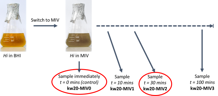
In their 2020 paper, Black et al., aimed to measure this competence response by switching happily proliferating Haemophilus influenzae in BHI medium, to a "starvation" medium called MIV. They took RNA at multiple time points and had cultures in triplicate to assess the deviation in response and enable statistical testing. We will focus initially on the control (t=0 minutes in MIV; kw20-MIV0) compared with t=30 minutes (kw20-MIV2).
Hopefully this all sounds quite familiar! If not, after this morning, make time to watch the videos we've generated to support these two workshops. These are embedded below and on the VLE.
You can also download the introductory slides here as a PDF.
Introduction to transcriptomics
How has the data in this workshop been processed so far?
What is a sequencing read?
The workshop
Set up your RStudio project
Start RStudio from the Start menu.
Make a new RStudio project. Put it in a sensible place with a sensible name. Remember that if you are using a university machine, select a location via the M/H drives, not just using the "Documents" shortcut. This will create problems for you!
Use the Files pane to make subdirectories for your raw_data, proc_data and plots. These names are suggestions only. Make a new script file, perhaps babs4_rnaseq_workshop.R, to complete your work.
Remember, you will eventually submit a single RStudio project which should represent the entire project over both workshops (3&4).
Access the data
During workshop 3 you will need 3 Haemophilus influenzae datafiles. Download and add to your raw_data subdirectory. From here on, Haemophilus influenzae will be abbreviated to Hi.
Hi_PRJNA293882_counts.tsv. These are the RNAseq data from Hi. The data includes 11 different conditions, each with three replicates (explained below). This is a tab separated file with sample names in the first row and feature IDs in the first column. The data are counts of the number of reads.
kw20 is the wildtype strain. OD600 is a measure of cell suspension density. Sxy is a transcription factor (encoded by tfoX) which regulates competence. The Sxy- strain is a null mutant strain where Sxy is non-functional.
| Condition | Strain | Media | OD600 | time (mins) | replicates |
|---|---|---|---|---|---|
| kw20-BHI1 | kw20 | BHI | 0.02 | NA | -F,-G,-H |
| kw20-BHI2 | kw20 | BHI | 0.60 | NA | -F,-G,-H |
| kw20-BHI3 | kw20 | BHI | 1.00 | NA | -F,-G,-H |
| kw20-MIV0 | kw20 | MIV | 0.25 | 0 | -A,-B,-C |
| kw20-MIV1 | kw20 | MIV | 0.25 | 10 | -A,-B,-C |
| kw20-MIV2 | kw20 | MIV | 0.25 | 30 | -A,-B,-C |
| kw20-MIV3 | kw20 | MIV | 0.25 | 100 | -A,-B,-C |
| sxyx-MIV0 | Sxy- | MIV | 0.25 | 0 | -A,-B,-D |
| sxyx-MIV1 | Sxy- | MIV | 0.25 | 10 | -A,-B,-D |
| sxyx-MIV2 | Sxy- | MIV | 0.25 | 30 | -A,-B,-D |
| sxyx-MIV3 | Sxy- | MIV | 0.25 | 100 | -A,-B,-D |
Hi_feature_names.tsv. This is a tab separated file with the Hi feature ID in column 1, the symbol for that feature in column 2 (if there is one, else "." is used as a placeholder), and a description in column 3 (vague at times!). There is a header.
Hi_feature_locations.bed. This is a tab separated file with a particular format called BED format. This means the columns have standard data types, so there is no header. Column 1 is the sequence a feature is located. Column 2 is the start position and column 3 the end position. Column 4 has the Hi feature ID. Column 5 has the biotype of the feature. Column 6 has the strand.
Load your libraries
We need the following packages for this workshop:
tidyverseWickham et al., 2019DESeq2Love et al., 2014EnhancedVolcanoBlighe et al., 2018ggplot2Wickham et al., 2016dplyrWickham et al., 2019 (this is part of tidyverse, but I always find loading it explicably helps with redundancy issues later on)
Note - this workshop is designed to run (and has been tested) on the managed University desktops. If you choose to run the workshop on your personal laptop, you may need to install additional packages. Remember that
install.packages() only works if a library a standard CRAN package. For DESeq2 and EnhancedVolcano, this is not the case - see guidance below. Update your version of R/RStudio before attempting to install new packages for the workshop.Remember - you can use the University of York Virtual Desktop Service to connect to a managed machine from your laptop to get the same experience of a managed machine from the comfort of your own laptop/desktop.
Open this if you're attempting installations on your own laptop.
I thoroughly advise you to use a managed machine or the virtual desktop service - this will make life easier! If you choose to go ahead on your own machine, read on.Update your version of R and RStudio.
tidyverse, ggplot2 and dplyr can be installed simply using the install.packages() built-in installer.Remember, installations are not instantaneous! The console (the window at the bottom left of RStudio) shows you when processes are still ongoing. The cursor will return when the process is done. So, if R/RStudio is asking you for information, such as whether or not you want to update other libraries etc. you need to answer this before running another line of code, otherwise R will keep waiting and waiting. Read the output - often you can skip updating other packages. This is far quicker for sure. Some updates may take >40 minutes and you won't be able to do anything else on RStudio until this is done.
Both
DESeq2 and EnhancedVolcano cannot be installed successfully with install.packages(). For DESeq2, you need to first install BiocManager, then load the BiocManager library, then use BiocManager to install DESeq2, then load the DESeq2 library:
   install.packages("BiocManager")

   library(BiocManager)

   BiocManager::install("DESeq2")

   library(DESeq2)
You need to install EnhancedVolcano using the remotes package and remotes::install_github() as in the main material above.Good luck!
# load these libraries
library(tidyverse)
library(DESeq2)
library(ggplot2)
library(dplyr)
library(EnhancedVolcano)

# if EnhancedVolcano is not found as a package, do the following:
install.packages("remotes")
library("remotes")
# press enter to skip updates when prompted
remotes::install_github("kevinblighe/EnhancedVolcano")
library(EnhancedVolcano)
Load datasets
# counts data
counts <- read.table("raw_data/Hi_PRJNA293882_counts.tsv", row.names = 1, header = TRUE)

# feature IDs and symbols where possible
featname <- read.table("raw_data/Hi_feature_names.tsv", row.names = 1, header = TRUE)

# feature locations, setting the column names for BED format
featlocs <- read.table("raw_data/Hi_feature_locations.bed", header = FALSE, col.names = c("chr","start","end","feat_ID","biotype","strand"))
Explore the datasets
Take some time to explore the data using view(), summary() and head(). Does the data look right? Do the column names make sense? Do you understand what each file is showing you?
Let's start to see what the data looks like, and how we can bring the datasets together.
# explore the counts data by making a histogram of the read counts in the first column
counts |> ggplot(aes(x = kw20.BHI1.F)) + geom_histogram()
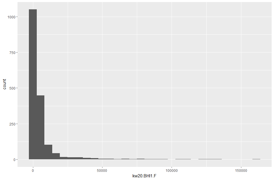
What is this histogram telling you about the distribution of read counts in this sample?
Most features have a "low" read count. But a few features have very high read counts.
So how can we make the plot easier to interpret?
# try a log10 transform of the same column
counts |> ggplot(aes(x = log10(kw20.BHI1.F + 1))) + geom_histogram()

# we do +1 inside the transform because log10(1) is 0
# this means the graph is not impacted by 0s and small decimals (missing and negatives respectively)
# less of a problem here because read counts are integers, but it may be relevant later on.
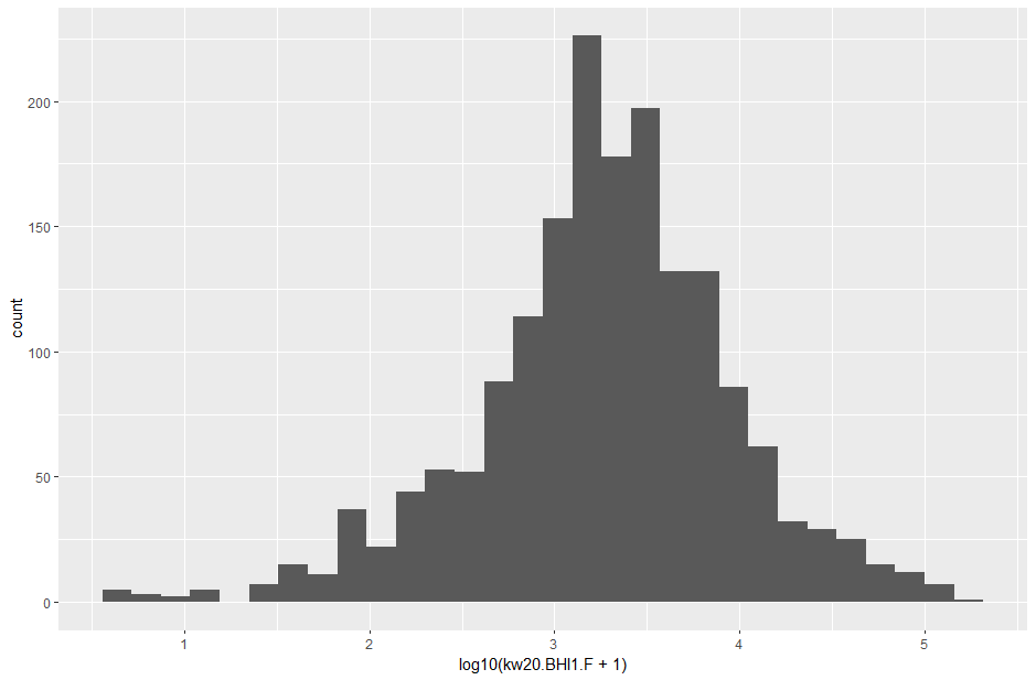
Much clearer! The count data has a fairly normal distribution with the means just above a thousand counts (103 on the x axis).
Now let's explore the other two datasets we loaded in.
# take a look at the top of the feature ID file with symbols and gene descriptions
head(featname)

# OK, so we get some symbols - maybe we can look for the muA, muB and gam genes we have been working on?
# use grep (pattern matcher) to check the symbol column for the three genes
featname[grep("muA|muB|gam", featname$symbol),]

# Success!
# those IDs suggest the features are quite close together. Let's use the location data to check.
# use the same pattern match as before, but extract the IDs and use them as a search term in the location data
mu_feats <- rownames(featname[grep("muA|muB|gam", featname$symbol),])
mu_feats_grep <- paste(mu_feats, collapse = "|")
featlocs[grep(mu_feats_grep, featlocs$feat_ID),]

# Yes - very close together
# in the BLAST/PHASTER workshop we were trying to annotate the prophage region annotated by PHASTER - we can use the location data now to speed this up
# use the coordinates from PHASTER (data workshop 2) to extract all IDs in the region
hi_prophage_region <- featlocs |> filter(between(start, 1558774, 1597183))

# think how you can use the code above to take these IDs from the prophage region to extract the gene symbols
# this will help your annotation of the prophage region from last session

# so now we have counts and feature IDs for genes we care about - what does gam look like?
# filter the counts data for the gam feature ID, transpose to turn the row into a column, and then convert back to a dataframe
gam_counts <- counts |> filter(row.names(counts) %in% c("gene-HI_1483")) |>
  t() |>
  as.data.frame()

# set the column name
colnames(gam_counts) <- "gamcounts"

# plot
ggplot(gam_counts, aes(x = rownames(gam_counts), y = gamcounts)) +
  geom_bar(stat = "identity") +
  scale_x_discrete(guide = guide_axis(angle = 90)) +
  labs(x = "samples", y = "Hi gam total reads")
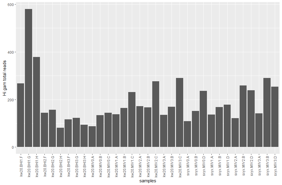
Great - we've already started to explore one of our genes of interest. But, we can't just compare raw counts on their own.
Why not? (Hint: are there any patterns in the bar chart related to the samples?)
There are patterns of high/low/medium etc across the replicates. We don't know whether this is biological or technical at this point.
But, before we can compare between genes, we need to know if each sample was sequenced to the same total depth (i.e. total number of reads). Otherwise, samples with more reads may just have higher counts - there may be no biological difference. Let's check.
# create a dataframe with sums for each column
count_tots <- data.frame(colSums(counts))
colnames(count_tots) <- "sum"

# let's check the ratio between the highest and lowest total read counts
max_reads <- max(count_tots$sum)
min_reads <- min(count_tots$sum)
max_reads / min_reads

# the highest has almost 4x as many reads as the lowest - no wonder there were differences in our last bar chart

# plot all the read totals to look for variance
ggplot(count_tots, aes(x = rownames(count_tots), y = sum)) +
  geom_bar(stat = "identity") +
  scale_x_discrete(guide = guide_axis(angle = 90)) +
  labs(x = "samples", y = "total reads")
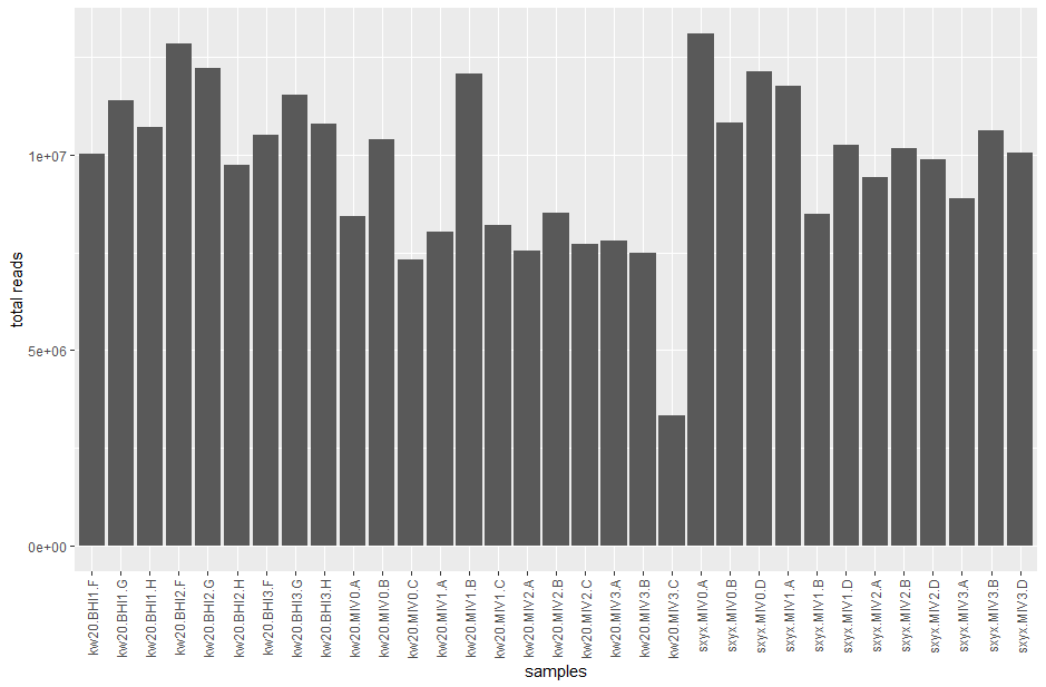
When we run differential expression analysis (DEA) later, DESeq2 accounts for the differences in read counts automatically. But, when we want to plot individual genes and make nice graphs we need to normalise the data. We are going to convert our read count data to TPM - transcripts per million.
I briefly covered TPM in the Introduction to Transcriptomics video, but I also have a specific video on RNAseq units if you want to know a bit more.
Normalise the count data
Normalising count data gives us a fairer way to compare between samples and even between genes in the samples.
What three things influence the read count for any feature?
The TPM of any feature can be calculated by:
- dividing the feature counts by the feature length (i.e. counts per base)
- dividing counts/base by the total counts for the sample
- multiplying by 1 million to get numbers we can work with (otherwise everything is very small)
#[EDIT] - do not subset the counts, instead work on the full dataset # let's first subset our data to only our core comparison: the impact of starvation media on Hi
#core_counts <- counts |> select(starts_with("kw20.MIV"))

# we have the position information on all features in featlocs, so we can create a new column for the feature lengths
featlens <- data.frame(mutate(featlocs, feat_len = (featlocs$end+1)-featlocs$start))
rownames(featlens) <- featlens$feat_ID

# we now need to combine our datasets so we can divide the feature counts by feature lengths for each sample
# to join two datasets you need a key to link associated data together
# that's why we've made the rownames the feature IDs (feat_ID) in both dataframes (hence column 0 in the merge)

#[EDIT] - we haven't created a core_counts subset now, so just use the full counts dataframe
#withlens <- merge(core_counts, featlens, by=0)
withlens <- merge(counts, featlens, by=0)
rownames(withlens) <- withlens$Row.names

# create a new dataframe with the sample counts divided by the lengths
#[EDIT] - we haven't created a core_counts subset now, so just use the full counts dataframe
#counts_per_base <- subset(withlens, select = colnames(core_counts)) / withlens$feat_len
counts_per_base <- subset(withlens, select = colnames(counts)) / withlens$feat_len

# now we use apply() to divide each value by the sum of its column, then multiply by a million to make it TPM
# the 2 indicates the function is applied on columns, rather than rows (where it would be 1)
tpms <- data.frame(apply(counts_per_base, 2, function(x){(x/sum(x))*1000000}))

# check each column now totals 1 million
colSums(tpms)

# round the data to 2 decimal places to make it more human readable (does each column still total 1 million?)
tpms <- round(tpms, 2)

# now, let's make a quick assessment as to how consistent TPMs and counts are with each other, using gam
# extract just the gam TPMs, as we did with counts above
gam_tpms <- tpms |> filter(row.names(tpms) %in% c("gene-HI_1483")) |> t() |> as.data.frame()
colnames(gam_tpms) <- "gamtpms"

# merge the TPM and count gam subset dataframes and plot as a scatter
gamcor <- merge(gam_tpms, gam_counts, by=0)
rownames(gamcor) <- gamcor$Row.names

ggplot(gamcor, aes(x=gamtpms, y=gamcounts)) +
  geom_point() +
  geom_text_repel(label=rownames(gamcor)) +
  labs(x = "gam TPMs", y = "gam read counts") +
  ylim(0, max(gamcor$gamcounts))

# ggrepel should have been installed/updated with EnhancedVolcano, if not, do this:
install.packages("ggrepel")
library(ggrepel)
# then rerun the block of code above

# calculate the correlation
cor(gamcor$gamcounts, gamcor$gamtpms, method = c("pearson"))
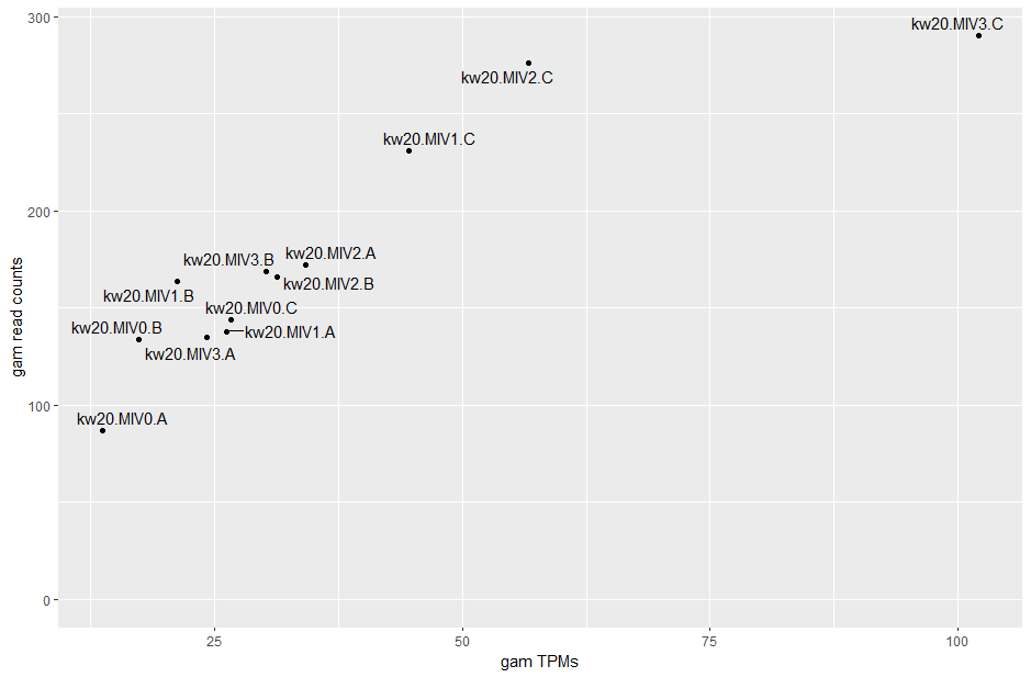
The correlation is pretty good for this gene (and it's usually quite good), though both MIV0.A and MIV3.C have quite different TPMs to what their read counts might indicate.
Principal component analysis
Before we do our stat testing for differences between conditions, it is always a good idea to perform principal component analysis (PCA).
Our data is "high dimensional data", because we have lots more rows than we could plot simultaneously to describe the samples. We can just about interpret plots on 3 axes, but no further. PCA is a method for "dimension reduction". It works by looking at correlated variance across the samples in each row of data. In biology this is quite easy to rationalise. Genes work in pathways, or may be regulated by the same transcription factor, so you can imagine that these genes would go up and down in expression together (i.e. they are not each truly independent measures of the samples). This means you can reduce your data to a smaller number of "principal components" where correlated measurements are collapsed together. You can then plot the most informative principal components (i.e. those accounting for the most correlated variance in the data) to get a feel for how your samples group together (or not).
The important thing here is that differential expression (like with any stat test) is only able to detect significant changes if your data are not too noisy (i.e. high in variance). So if your samples do not group together nicely by PCA it may be informative for removing samples (outliers) or explain why some comparisons will not give significant differences.
Hopefully this becomes clearer with a plot.
# perform PCA on the tpm dataframe
#[EDIT] - previously this was just for the kw20.MIV* samples. Running on the full set is fine but will change the plot below
#res_pca <- princomp(tpms)
# we will subset the data here just to our core kw20.MIV samples
kw20MIV_tpms <- tpms |> select(starts_with("kw20.MIV"))
res_pca <- princomp(kw20MIV_tpms)

# extract the variance accounted for by each principal component (squared standard deviation as proportion of total)
pca_var <- round((data.frame(res_pca$sdev^2/sum(res_pca$sdev^2)))*100,2)
colnames(pca_var) <- "var_perc"
pca_var

# most of the variance is accounted for by PCs 1 and 2. You can now plot a scatter of these samples to see if they group based on these components
# extract PCs 1 and 2
pca_comps <- data.frame(res_pca$loadings[, c("Comp.1", "Comp.2")])

# create axis labels which include the % variance accounted for by each component
pca_x <- paste(c("PC1 ("), pca_var["Comp.1",], c("%)"))
pca_y <- paste(c("PC2 ("), pca_var["Comp.2",], c("%)"))

# scatter
ggplot(pca_comps, aes(x=Comp.1, y=Comp.2)) +
  geom_point() +
  geom_text_repel(label=rownames(data.frame(res_pca$loadings[, 1:2]))) +
  labs(x = pca_x, y = pca_y)

# you could plot PC1 vs PC3 or PC2 vs PC3 to further interogate the data and the relationships
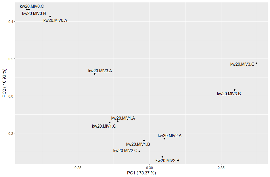
What does this plot tell you about the samples?
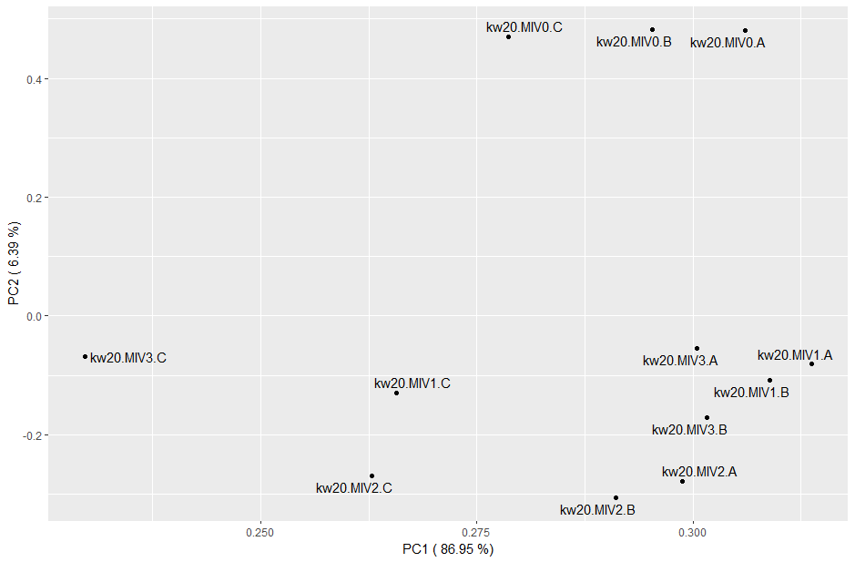
Genes with higher expression also have higher variance, so a log transformation will reduce that weighting. Try rerunning the PCA code with: res_pca_log10 <- princomp(log10(tpms+1))
Does the log transformation give a different result, or tell you anything new about the data?
The log transformation strongly suggests that the "C" replicates across conditions were quite different to the rest. It's possible these were processed all at the same time, different to those of A and B, maybe even by a different person. We may be able to control for this technical artefact during differential expression.
Your PCA plots would be good ones to save. Make sure you give them sensible names and put them in your plots directory to keep things organised.
You can use the Export function on the Plots pane of RStudio, or code it. See below the PCA image.
ggplot(pca_comps, aes(x=Comp.1, y=Comp.2)) +
  geom_point() +
  geom_text_repel(label=rownames(data.frame(res_pca$loadings[, 1:2]))) +
  labs(x = pca_x, y = pca_y)
ggsave("plots/tpm_pca.pdf")
Differential expression analysis
We're now going to focus in on the main comparison for this workshop: the impact of the changed media after 30 mins (i.e. comparing t=30 against t=0; MIV2 vs MIV0).
# reduce counts matrix to just the groups we want
comp_counts <- counts[, grep("kw20.MIV0|kw20.MIV2", colnames(counts))]

# DESeq2 needs a dataframe detailing the experimental setup
sample_info <- data.frame(colnames(comp_counts))
colnames(sample_info) <- c("sample")
rownames(sample_info) <- sample_info$sample
sample_info

# currently sample_info looks very sparse, but we actually have all the information we need because of our consistent sample naming
# we can split the sample name and this gives us the genotype (kw20), condition (MIV0, MIV2) and replicates (A,B,C)
sample_info <- sample_info |> separate(sample, c("genotype", "condition", "replicate"))

### during the workshop, some people working on personal machines had issues with the separate() command
### this is part of tidyverse, so make sure that is loaded and updated, and try again
### if that still doesn't work, see the base R (i.e. no libraries needed) one-liner solution which replaces the 5 code lines above
### sample_info <- read.table(text=gsub("[.]", ",", colnames(comp_counts)), sep=",", col.names=c("genotype", "condition", "replicate"), row.names = colnames(comp_counts))

# crucial check needed now - are the columns in the counts data all found in the rownames of the sample_info (and in the same order)
all(rownames(sample_info) %in% colnames(comp_counts))
all(rownames(sample_info) == colnames(comp_counts))

# these are both TRUE, which is good. If these are FALSE, you need to reorder your columns/rows to make them match

# now we can run the differential expression
# the design parameter tells DESeq2 what comparison you want to make
dds <- DESeqDataSetFromMatrix(countData = comp_counts, colData = sample_info, design = ~ condition)

# explicitly set the control condition so fold changes are in the direction you want/makes biological sense
dds$condition <- relevel(dds$condition, ref = "MIV0")

# run DESeq2
dds <- DESeq(dds)
dds_results <- results(dds)

# get some quick summaries of 'significant' changes and take a look at the results
summary(results(dds, alpha=0.05, lfcThreshold = 1))
dds_results
Good news! There are lots of significant changes. We use as log2 fold change as it makes positive and negative changes symmetrical - see the table below for an explainer. We also need to have an 'adjusted' p value, not just the normal p value. The adjustment accounts for multiple testing of the data, where chance differences could come through as false positives. Effectively the adjustment makes our threshold for significance more stringent.
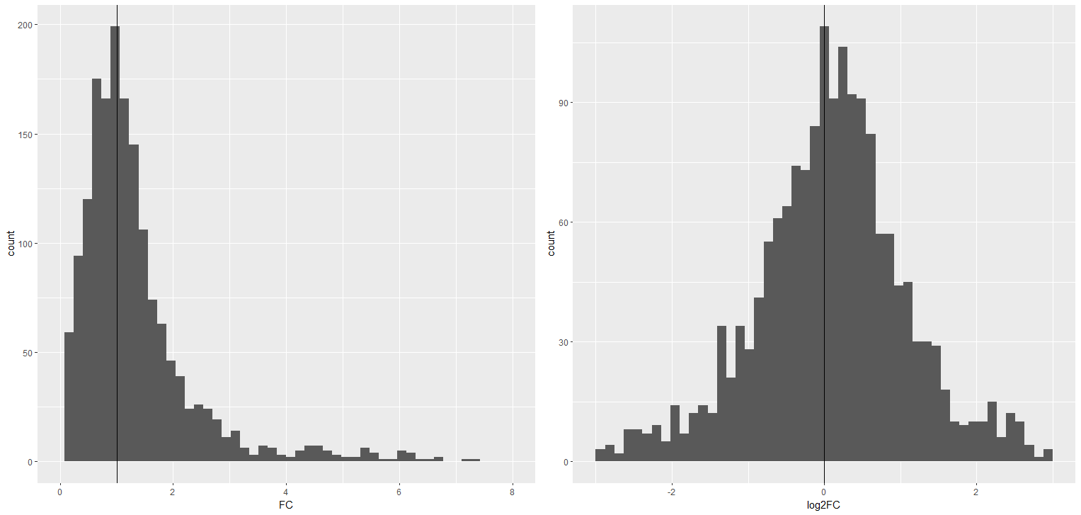
When we compare values in two groups, we divide our experimental group by our control group to generate fold change values. So if something goes up in the experimental group, fold change will be greater than 1. Doubling expression or halving expression should be equivalent in our heads (they are reciprocal values), but they differ in their arithmetic distance from 1 (see the table). This means increasing expression could have a fold change value from >1 all the way to infinity. But a decrease can only go from <1 to approaching 0 - see the left histogram below.
A log2 transformation of the fold change brings the equivalence back, making it symmetrical around 0 (see right hand histogram). This is why volcano plots use a log2 x axis.
| gene | testavg TPM | controlavg TPM | test/control | log2(test/control) |
|---|---|---|---|---|
| geneA | 100 | 50 | 2 | 1 |
| geneB | 50 | 100 | 0.5 | -1 |
| geneC | 20 | 20 | 1 | 0 |
That's the maths explainer over. Let's get back to interrogating the results of our DEA.
# currently our results all have the feature ID, so let's add in the gene symbol and TPMs
# first merge with the featnames to get symbols
dds_results <- merge(as.data.frame(dds_results), featname, by=0)
rownames(dds_results) <- dds_results$Row.names
dds_results <- dds_results[,-1]

# then subset the TPMs, calculate log2FC and merge together
comp_tpms <- tpms[, grep("kw20.MIV0|kw20.MIV2", colnames(tpms))]
comp_tpms <- mutate(comp_tpms, MIV0_avg = rowMeans(select(comp_tpms, contains("MIV0"))),
                    MIV2_avg = rowMeans(select(comp_tpms, contains("MIV2"))))
comp_tpms <- mutate(comp_tpms, log2FC = log2((MIV2_avg+1)/(MIV0_avg+1)))
comp_red_tpms <- comp_tpms |> select(-starts_with("kw20.MIV"))

dds_tpm <- merge(dds_results, comp_red_tpms, by=0)
rownames(dds_tpm) <- dds_tpm$Row.names
dds_tpm <- dds_tpm[,-1]

# we now have log2FC values calculated from the DESeq2-normalised counts and our TPMs
# are they well correlated?
cor(dds_tpm$log2FoldChange, dds_tpm$log2FC, method = c("pearson"))

# now you have some context (particularly gene names), order by most significant and take a look at the top 20
head(dds_tpm[order(dds_tpm$padj),], 20)
Are there genes here which make sense?
The com genes are competence genes, so that makes a lot of sense. We also have DNA (dprA) or recombination (rec2) regulators.
There are also lots of genes without symbols. This is fine! It may represent new biology to explore. Some of the descriptions for these unnamed ones make sense though - protein transport etc.
Looking at a table like this is tricky, so let's make a volcano plot!
# first extract a list of genes (with symbols) to annotate the biggest changes on our volcano
# subset the dataframe where the symbols column does not equal "."
# we need the square brackets here otherwise "." takes on its special meaning of "match any character"
withsymbols <- dds_tpm[- grep("[.]", dds_tpm$symbol),]

# take the top 60 based on absolute log2FC (so this includes big negatives if there are any)
siggenes <- head(withsymbols |> arrange(desc(abs(log2FC))), 60)$symbol

# make the volcano plot - you can personalise these forever, check out - https://github.com/kevinblighe/EnhancedVolcano
# the cutoffs define the dotted line thresholds and default colours
# the second line is all about the labels used
# the third line are some personal preferences on the plot layout - play with these!
EnhancedVolcano(dds_tpm, x = "log2FC", y = "padj", FCcutoff = 1, pCutoff = 0.05,
                lab = dds_tpm$symbol, selectLab = siggenes, labSize = 4.5, max.overlaps = 1000, drawConnectors = TRUE,
                legendPosition = 0, gridlines.major = FALSE, gridlines.minor = FALSE)

# there are a lot of big, significant changes in this dataset - I would perhaps suggest making the FCcutoff harsher. The plot below is for 2.5
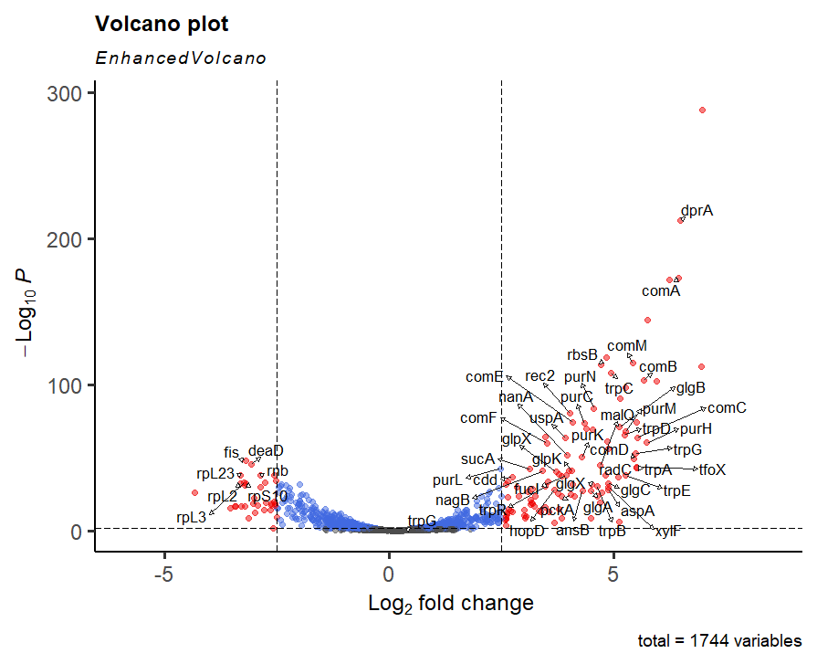
The volcano plot highlights the large number of very significant changes in the dataset after culture in the starvation media, MIV. We've already mentioned some of the genes such as dprA and comA. Next session we will work more on exactly what the biological impact is, but for now investigate a few more of the groups. This can be from the description column in the results, or by some tactical research on google.
What do the pur and trp genes do?
Genes such as purC are involved in making nucleotides. Similarly, genes like trpC make the amino acid tryptophan. MIV lacks both of these metabolites.
Don't forget about the downregulated genes - any common themes?
The rpL and rpS genes encode the large and small ribosomal subunits. fis activates rRNA transcription. It looks like there is a general downregulation of translation machinery.
Do you recognise tfoX?
tfoX encodes the Sxy protein which is involved in competence response (directly via CRP). It is upregulated here and we have another Hi dataset which has a Sxy null mutant. Can you make any hypotheses about what may happen in Sxy mutants when they are grown in MIV?
What about muA, muB and gam?
They don't come up in this most significant list. You could change the siggenes variable to include only these genes and see where they are on the volcano. Or use your grep commands from earlier in the workshop to extract these genes from the results file.
Modest but statistically significant upregulation is seen across all genes. So there is constituitive expression, enhanced in MIV.
Finishing up for today
Fantastic work! Lots of R coding and you've taken a big dataset, normalised it, extracted the columns you're biologically interested in, and performed differential expression analysis. Next session you'll be focused on what this actually means, relating this to genome location and how these genes may be regulated through regulons. Before that you need to make sure you've got everything saved so you don't need to do it again.
Make sure you have saved the plots you want to save - particularly the PCA and volcano plots - and also the relevant datasets which you've modified.
write.table(dds_tpm, file="proc_data/MIV0vsMIV2_DEA_full_results.tsv", sep="\t", row.names=TRUE)
write.table(tpms, file="proc_data/full_dataset_TPMs.tsv", sep="\t", row.names=TRUE)
write.table(comp_tpms, file="proc_data/MIV0vsMIV2_TPMs.tsv", sep="\t", row.names=TRUE)

# and anything else you've done which is relevant to you
GREAT WORK! See you next week!
Consolidation and extending the workshop analysis (if you’re interested)
If you want to check your understanding, the best bet is to look back through the workshop section headers and make sure you understand what each step was for. It's easy to put your head down and ignore the biology - so always bring it back to that. Remember, the question was how Haemophilus influenzae, a naturally competent bacterium, would respond when placed in starvation conditions and what this says about the regulation of the competence response.
You will need to weave the RNAseq data analysis into your project report. So, how does this data support your wet lab work, and the BLAST/PHASTER practical in data workshop 2? How does it fit together? Can you check the wet lab results in the RNAseq data?
There is also the opportunity to use the other datasets available to you to further explore these questions, and to explore the data more too.
One outstanding question is why the C replicates were so different from the rest (look back at your PCA plots). I mentioned that we might be able to control for this difference. Let's take a look.
# revisit the DEA section - we're going to run another type of DEA
# we can include the replicate information (which is in sample_info) to control for variance based on the replicate
# when we instruct the DEA design, put variable you want to control before the experimental variable you want to measure
dds2 <- DESeqDataSetFromMatrix(countData = comp_counts, colData = sample_info, design = ~ replicate + condition)

# you can then follow the rest of the analysis we did, include summaries and making the volcano plot
Often we control for replicate if there is a genuine reason to do so, such as replicates coming from different labs, isolates or donor backgrounds. In this case, "C" is not really a separate grouping and we don't know for certain it was treated differently - this may simply reflect genuine biological variance (rather than a technical annoyance). We do get a few more significant hits, but we already had more significant hits than we could feasibly validate in the lab, so it's unlikely we've gained anything properly new.
However, we can flip the DESeq2 design to work out what it was about the replicates that caused the variance on the PCA.
If you try this, you'll see that lots of ribosomal RNA comes up as significant. Remember, our dataset was derived after rRNA depletion, so any rRNA leftover is simply a measure of how (in)efficient the library prep was. It looks like the C samples had a worse prep, and therefore have more rRNA leftover, hence the variance on the plot. Again, we have lots of significant results despite this, but a solution could be to remove any rRNA genes from the count matrix, removing this problem. There is a good reason to do this. The danger is overdoing it. This is where good data management and note taking comes in.
Another good question is whether the response we see at t=30 happens earlier (MIV1; t=10) and/or is maintained (MIV3; t=100). Things you now have the skills to answer.
Could you make sensible hypotheses about the other datasets you have access to, that may also help your understanding of the Hi competence response under stress? I look forward to seeing what you might come up with...
Return to tutorial introduction.
Video explainers
Introduction to transcriptomics
This video was included in the week 4 teaching materials on the VLE to view before the workshop - hopefully this is just here as a reminder. Here we introduce you to some of the concepts of transcriptomics - where the data comes from, what it looks like, and what you'll be doing with it in the data workshops.
Return to tutorial introduction.
Begin the workshop.
Data processing before this workshop
This video was included in the week 5 teaching materials on the VLE to support the workshop material. We introduce you to the data you will analyse in these two data workshops (3 and 4), and tell you what has happened to go from raw sequencing data (files for each sample total c.40 million lines) to the counts matrix you will work on (1745 rows and 6 columns, in the first instance).
Return to tutorial introduction.
Begin the workshop.
What is a sequencing read
This video was included in the week 6 teaching materials on the VLE to support the workshop material. We had some confusion as to what a sequencing read actually is - so hopefully this explainer helps.