Mason Lab BSc project - Multiomic analysis of bladder cancer
This site contains helpful information for completing your 28H final year BSc dissertation project in the Mason Lab. General information on the module is available on the VLE - check this regularly.
Expectations, meetings and assessments
Across the year you are expected to spend 1.5-2 days per week on your project, balancing this 40 credit module with your other module topics. As this is a data project, you can be very flexible with when you are working. Remember, this is an individual project (and must be completed and submitted independently), but it is likely the other students who also selected this topic will face similar issues, so support each other! You may enjoy arranging to meet in a computer lab or in the library at the same time in small groups. Whatever works for you.
28H does have some workshops, so make sure you check the Module Planner on the VLE site and look out for any announcements from the module organiser. There is a useful checklist of expectations available here.
During semester 1, we will have our group supervision meetings on Wednesdays 2-3 in B/M/049. Some particular dates to note are tabled below:
| Week | Date | |
|---|---|---|
| S1 W2 | W 01/10/25 | First group supervision meeting |
| S1 Consolidation Week | W 29/10/25 | No supervision meeting |
| S1 Week 6 | T 04/11/25 | Bookable one to one slots with Andrew - emailed on 24/10 |
| S1 Week 8 | W 19/11/25 | Formative presentations - emailed on 24/10 |
| S1 Week 11 | W 10/12/25 | Last meeting of semester - bookable one to one slots with Andrew - email coming on 24/11 |
| S2 Week 1 | w/c 09/02/26 | First supervision meeting of semester 2 (day/time TBC) |
| S2 Week 6 | w/c 16/03/26 | Final supervision meeting of project (day/time TBC) |
As your project develops I will set aside an open office hour where I will be available in case you want to drop in to discuss your project. This will be on a first come, first served basis or via bookable slots.
The main assessment is your 4000 word scientific report. Deadline: Tuesday 5th May at 12 noon (S2 W11).
There is also the formative oral presentation in semester 1 (S1 W8). There are multiple opportunities for feedback on your writing (S2 W0, S2 W8) - these are for you to make the most of, and are not compulsory.
Scope and aims of your project
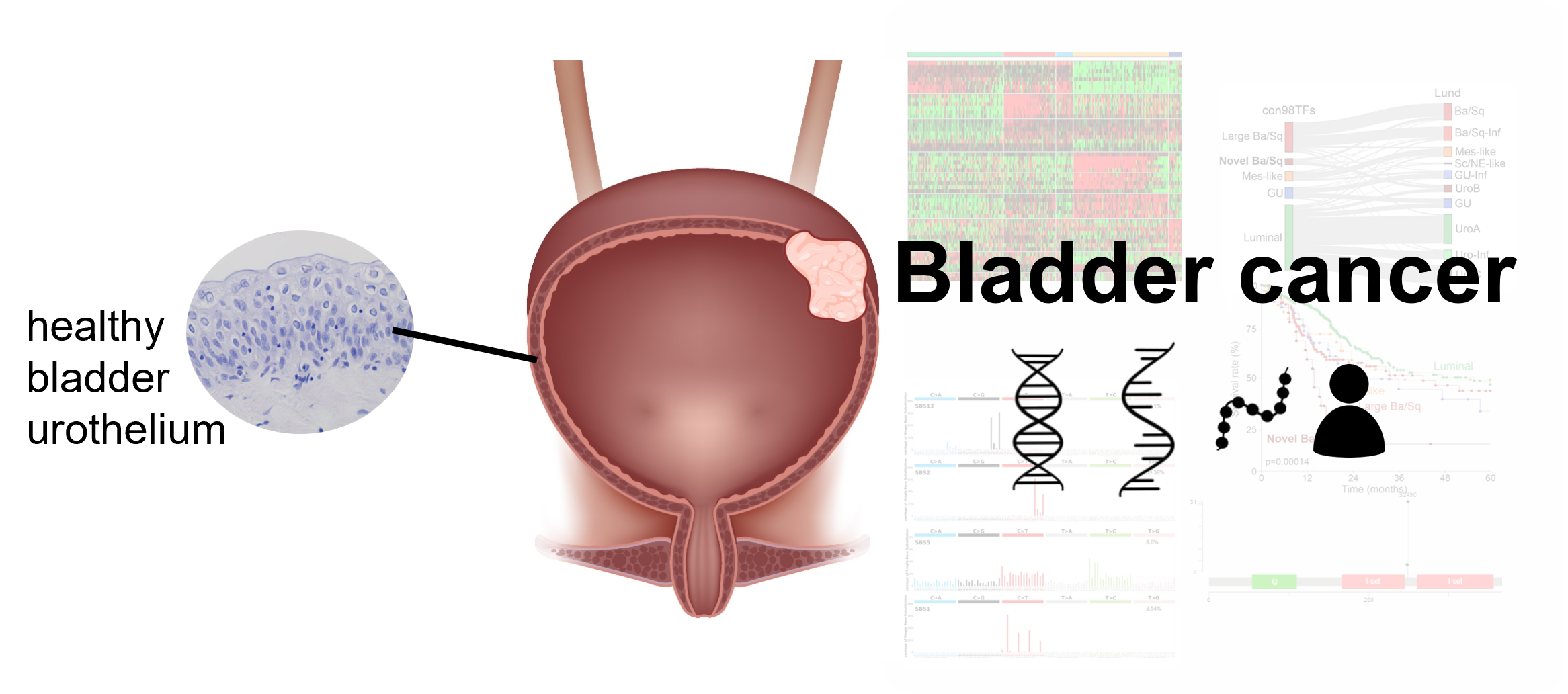
Bladder cancer is an incredibly diverse disease, characterised by a very high mutational burden and the highest number of different driver genes among solid cancers. The challenge is to understand the drivers in each patient’s cancer so that we can select, repurpose or develop more personalised treatment.
In this project you will use different types of sequencing data generated from 408 advanced bladder cancers included in The Cancer Genome Atlas (TCGA), an international programme built to understand over 30 different cancer types from over 10,000 patients. Whilst the power of TCGA was having multiple data types, most studies have only looked at one. In your project you will combine datasets to better understand the impact of mutations and gene expression changes on bladder cancer biology. The overall aim of my lab is to better understand existing bladder cancer subtypes, or to find new subtypes which could have a route to clinic.
So, how about your project? You will do the following:
- Familiarise yourself with muscle-invasive bladder cancer literature
- Devise a relevant, sensible and testable investigation where you can compare different types of muscle-invasive bladder cancers using the multiple data types you have available to you
- Perform a systematic data investigation to answer your question
- Critically review your results and determine how this fits within the wider literature - what have we learned and is it clinically relevant?
- Consider and plan the future work you would propose to further understand your results and their relevance (incl. wet lab work, further data analysis, clinical follow up etc.)
Coming up with your own study might feel daunting just now, but don't worry - there are some useful starting points below including some key papers. If you are doing the Cancer cell & molecular biology module, or the Genomics module, you should get some useful context and help from lectures and workshops - don't worry if you don't take either of these. A minimal project would be to identify tumours with/without a mutation in a relevant cancer gene, and then to use RNA sequencing data to compare the gene expression profiles of these cancers, and to try and work out what that means. We have lots of different data (and there are >400 cancers in the dataset) so the project can grow, develop, extend in lots of different ways - the best approach is to try and find a question where you'd be interested in finding out the answer.
Something you won't have maybe thought about too much before is the ethics of working with human genomic data. We'll speak about this during our sessions, but your project work is covered under an existing ethics approval from the Biology Ethics Committee.
Getting help with your project
First thing to remember is that you are doing new research. This means we don't necessarily know the "right" answer when it comes to checking your results. Make sure you are checking your scripting and that you are really critical of your results - do they actually make sense?
We expect you to have a good go at solving problems and troubleshooting, but don't get stuck for too long without asking for help. Work with the rest of the group (they're working with the same data too). If you still need help you can use the google form embedded below to (anonymously, if you like) ask for help, but do check the existing questions and responses first on this google sheet. Marcello (bioinformatician in my lab) or I will pick these up, typically within a working day, so check back regularly.
Introduction to bladder cancer
To get you started I've recorded a mini lecture on muscle invasive bladder cancer. This is enough to get you going, but you'll want to dig deeper in areas relevant to your project (including looking at studies from other cancer types). Remember - what I've said is my scientific assessment based on the literature and my own research experience - your critique is welcome and expected!
Download slides in pptx or PDF formats.
Relevant (big) starting papers
Robertson et al, 2017, Cell - the paper which describes the full TCGA MIBC cohort
Kamoun et al, 2020, European Urology - the paper which introduces the MIBC "consensus classifier"
Shi et al, 2020, Genome Medicine - the paper which describes bladder cancer hotspot mutations, particularly those created by APOBEC mutagenesis
Baker et al, 2022, Oncogene - paper from our unit which attempts to link viral infection to bladder cancer
Martincorena et al, 2017, Cell - paper identifies recurrent driver genes across all cancers in TCGA - see Figure 2
Cotillas et al, 2024, The Journal of Molecular Diagnostics - an alternative view to bladder cancer classification (all disease stages)
The data
This google drive contains major data files from The Cancer Genome Atlas muscle invasive bladder cancer cohort. We have pre-processed some of these to make them less difficult to work with, but some of them are still very large! You can and should work with these in R. You can also open these in notepad (but use notepad++ because this has some actual functionality).
Most of the data files are tab spaced value (tsv) files which means you can open and process them easily (even in Excel if you want a quick look). The .maf, .gmt and .bed format files are tsv format files as well, but they are organised in a partciular way with particular columns in a particular order. A description of each file is given in the table below:
| Filename | Technology | Description |
|---|---|---|
| c2.all.v2023.2.Hs.symbols.gmt | annotation file | curated lists of genes involved in different pathways |
| CNA_gene-level-CN.tsv | copy number array | number of copies of each gene in each tumour (could represent segmental or casette alterations) |
| gc47_gene_locations.bed | annotation file | GRCh38 gene locations across the genome |
| h.all.v2023.2.Hs.symbols.gmt | annotation file | curated lists of genes involved in different “hallmark” pathways |
| methylation_CpG-array.tsv | 5mC methylation array | methylation intensity beta values between 0 (low) and 1 (high) |
| miRNA_counts.tsv | miRNA sequencing (short RNAseq) | raw read counts per miRNA gene |
| miRNA_CPMs.tsv | miRNA sequencing (short RNAseq) | counts per million to control for differences in sequencing depth |
| mRNA_gc47-counts.tsv | mRNA sequencing (polyA RNAseq) | raw read counts per gene feature |
| mRNA_gc47-TPMs.tsv | mRNA sequencing (polyA RNAseq) | transcripts per million to control for depth and feature length |
| mRNA_gc47-TPMs_ConsensusClassifier.tsv | sample annotation | Consensus classification of each tumour according to Kamoun et al (2020) |
| mRNA_gc47-TPMs_LundTax2023Classifier.tsv | sample annotation | Lund classification of each tumour according to Cotillas et al (2024) |
| oncoKB_2024-02-08.tsv | annotation file | list of human “cancer genes” curated by the oncoKB website |
| TCGA-BLCA-clinical-metadata.tsv | patient metadata | relevant metadata for patients and their cancer |
| WGS_coding-regions-only.maf | whole genome sequencing | mutations in tumours filtered to just include mutations in coding regions |
| WGS_mutation-in-at-least-4-patients.maf | whole genome sequencing | mutations in tumours filtered to only include mutations found in 4 or more patients |
| WXS.maf | whole exome sequencing | mutations in tumours identified by only profiling coding regions |
I've provided these datafiles so you can do your own specific analysis, including making your own versions of figures. There are places to get data summaries for this cohort, even some top-level analysis and figures. But these alone will not be enough for a good project mark. By coding it yourself you can ask good questions and get to grips with the data - allowing you to critique how and when it can (or should) be used (and when it really shouldn't).
Before jumping into the data analysis, do some reading to get a better feel for the cancer biology and the technologies I've talked about. Then you should use cBioPortal to do some initial playing with the data (in a browser). I've written a course (~2hours) on how to use cBioPortal, including with demos, problem solving tasks to get used to using the website, and then a worked coding example in R to demonstrate how to download and work with this type of data. This will be very (very) useful for your project - mix up your reading by completing my Intro to cBioPortal course in your own time.
Getting started with your analysis
So where to begin? Well, first, don't worry. You need to get some better understanding of bladder cancer, then you can start to work with the data more. I'm going to give a brief demo idea below which follows this experimental strategy:
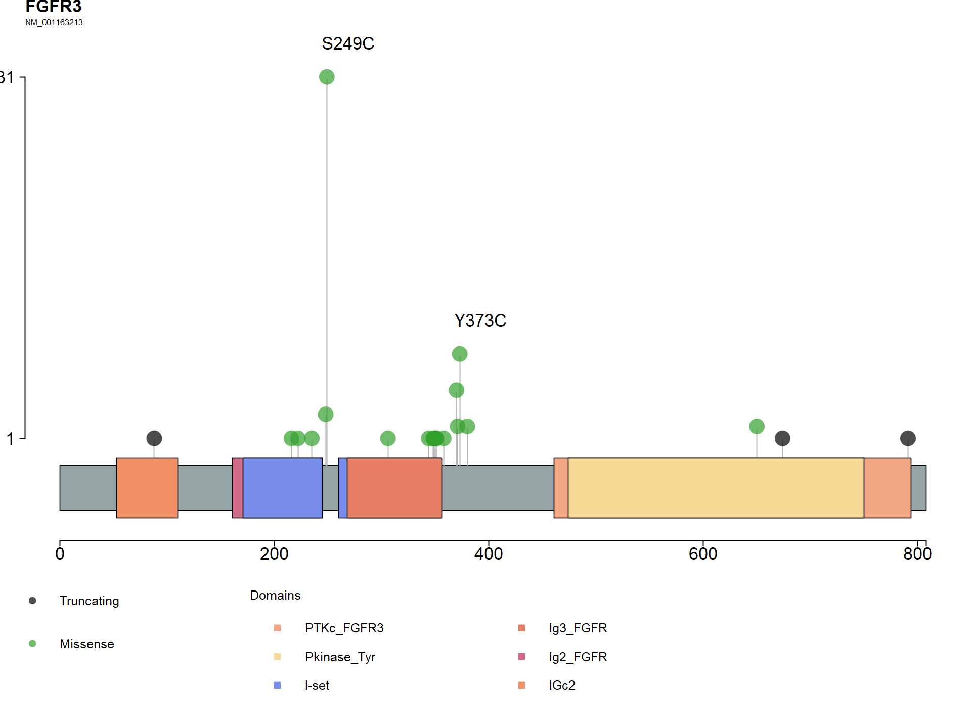
- Find tumours which have a mutation in FGFR3
- Run differential expression analysis between tumours with or without an FGFR3 mutation, but only in tumours within the LumP consensus classification
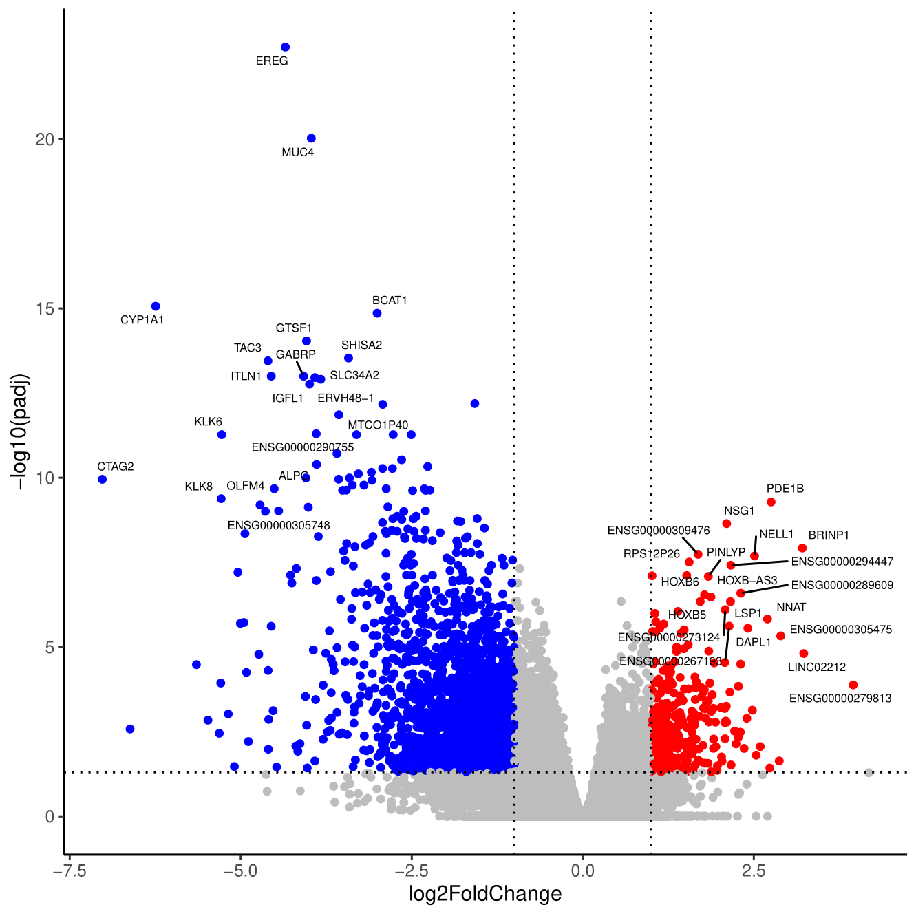
- Plot a labelled volcano plot
- Run gene set enrichment analysis to start to interpret the biology of the results
Remember, this is only an indicative starting point - your analysis would need to go deeper and to consider, graph, discuss and (where necessary) control for any confounding variables I have skipped over.
# load libraries
library(dplyr)
library(maftools)
library(ggplot2)
library(ggrepel)
library(DESeq2)
library(fgsea)
library(BiocParallel)

# enable parallel computing
register(SerialParam())


## Section 1 - identify tumours with FGFR3 mutation

# read whole exome sequencing MAF
wxs_maf <- read.maf("WXS.maf")

# get summaries of all mutated genes, get number of patients with FGFR3 muts
gene_tots <- getGeneSummary(wxs_maf)
gene_tots[grep("FGFR3", gene_tots$Hugo_Symbol),]$MutatedSamples

# produce a lollipop plot showing where the mutations in FGFR3 are
lollipopPlot(maf = wxs_maf, gene = "FGFR3", AACol = "Protein_Change", cBioPortal = TRUE,
             pointSize = 4, labelPos = c("249", "373"), labPosSize = 2,
             titleSize = c(2, 1), showMutationRate = FALSE,
             domainLabelSize = 2, showDomainLabel = FALSE,
             axisTextSize = c(2,2), legendTxtSize = 1.5, )

# extract FGFR3 mutant patient IDs
fgfr3_muts <- unique(wxs_maf@data[Hugo_Symbol == "FGFR3", Patient_Id])
## Section 2 - Load RNAseq data and subset to keep only LumP tumours, with FGFR3 genotype info

# load consensus classifiers for each tumour and keep only LumP tumours
# patient ID is in form TCGA-##-####, but individual samples (tumour, blood etc) have a label like -01A at the end
# the substr command is used to remove this to return to patient ID
con_class <- read.table("mRNA_gc47-TPMs_ConsensusClassifier.tsv",
                        header = TRUE, sep = "\t")
con_class$Patient_ID <- substr(con_class$ID, 1, 12)
lump_patients <- con_class$Patient_ID[con_class$consensusClass == "LumP"]

# keep only LumP tumours, with information on FGFR3 wildtype vs mutant
lump_fgfr3 <- intersect(fgfr3_muts, lump_patients)
lump_fgfr3_wt <- setdiff(lump_patients, lump_fgfr3)

# create a sample info dataframe for differential expression
sample_ids <- c(lump_fgfr3, lump_fgfr3_wt)

genotype <- c(rep("MUT", length(lump_fgfr3)),
              rep("WT", length(lump_fgfr3_wt)))

sample_info <- data.frame(row.names = sample_ids, genotype = genotype)

# load RNAseq count data, adapt column names and subset to only keep LumP tumours
counts <- read.table("mRNA_gc47-counts.tsv", check.names = FALSE,
                    header = TRUE, row.names = 1, sep = "\t")
colnames(counts) <- substr(colnames(counts), 1, nchar(colnames(counts)) - 4)

lump_counts <- counts[ , sample_ids]
lump_counts <- round(lump_counts[complete.cases(lump_counts), ])


## Section 3 - Differential expression
# how is gene expression different in (LumP) tumours with mutant or wildtype FGFR3?

# create the DESeq2 object
dds <- DESeqDataSetFromMatrix(countData = lump_counts,
                              colData = sample_info,
                              design = ~ genotype)

dds$genotype <- relevel(dds$genotype, ref = "WT")

# run DESeq2 - this will take a few minutes
dds <- DESeq(dds)

# store results
dds_results <- results(dds)

# in relevant columns, process NA values and apply a max adjusted p value
dds_results$log2FoldChange[is.na(dds_results$log2FoldChange)] <- 0
dds_results$padj[is.na(dds_results$padj) | dds_results$padj > 0.99] <- 0.99

# add labels for colouring the volcano plot
dds_results$DEA <- "NO"
dds_results$DEA[dds_results$log2FoldChange > 1 & dds_results$padj < 0.05] <- "UP"
dds_results$DEA[dds_results$log2FoldChange < -1 & dds_results$padj < 0.05] <- "DOWN"

# add gene symbols as column for easy plot labelling
dds_results$symbol <- rownames(dds_results)

# create pi values (fold change multiplied by stat significance) for later gene ranking
dds_results$pi <- dds_results$log2FoldChange * -log10(dds_results$padj)
dds_results_pi_sorted <- dds_results[order(dds_results$pi),]

# create reduced dataframe of most significantly different genes, for labelling
# using pi values means you prioritise most biologically significant
top_genes <- c(head(dds_results_pi_sorted$symbol, 20), tail(dds_results_pi_sorted$symbol, 20))
genes_to_label <- dds_results[dds_results$symbol %in% top_genes, ]

# create a labelled, coloured and annotated volcano plot
ggplot(dds_results, aes(x=log2FoldChange, y=-log10(padj))) +
  geom_point(aes(colour = DEA), show.legend = FALSE) +
  scale_colour_manual(values = c("blue", "gray", "red")) +
  geom_hline(yintercept = -log10(0.05), linetype = "dotted") + geom_vline(xintercept = c(-1,1), linetype = "dotted") +
  theme_bw() + theme(panel.border = element_blank(), panel.grid.major = element_blank(), panel.grid.minor = element_blank(), axis.line = element_line(colour = "black")) +
  geom_text_repel(size=2, data=genes_to_label, aes(x=log2FoldChange, y=-log10(padj), label=symbol), max.overlaps = Inf)

# save plot and data
ggsave("LumP_FGFR3_MUTvsWT_volcano.pdf")

write.table(dds_results, file="LumP_FGFR3_MUTvsWT_DEA_results.tsv",
            sep = "\t", row.names = FALSE, col.names = TRUE)
## Section 4 - gene set enrichment analysis (GSEA)
# this allows you to look for pathway-level changes, rather than having to google genes individually

# load MSigDB gene set
genesets = gmtPathways("c2.all.v2023.2.Hs.symbols.gmt")

# use pi values to rank genes from "most up" to "most down" in the comparison
prerank <- dds_results[c("symbol", "pi")]
prerank <- setNames(prerank$pi, prerank$symbol)
str(prerank)

# run fgsea
fgseaRes <- fgsea(pathways = genesets, stats = prerank, minSize=15, maxSize = 500)

# store top10 most enriched
# positive enrichment is "(relatively) up in the FGFR3 mutant tumours"
# negative enrichment is "(relatively) up in the FGFR3 wildtype tumours"
top10_fgseaRes <- head(fgseaRes[order(pval), ], 10)
top10_fgseaRes

# create bar chart of normalised enrichment scores (NES) for top10 hits
ggplot(top10_fgseaRes, aes(x = NES, y=reorder(pathway, -pval), fill = factor(sign(NES)))) +
              geom_bar(stat = "identity", width = 0.8) +
              labs(title = "GSEA", x = "Normalised Enrichment Score (NES)", y = "Pathway") +
              theme_minimal(base_size = 16) +
              scale_fill_manual(values = c("#0754A2", "#B10029"), guide = "none") +
              scale_y_discrete(labels = function(x) gsub("^HALLMARK_", "", x)) +
              theme(axis.text = element_text(color = "black"),
                       axis.title = element_text(color = "black"),
                       panel.grid.major = element_blank(),
                       panel.grid.minor = element_blank())

ggsave("LumP_FGFR3_MUTvsWT_top10_c2-GSEA.pdf", width=16, height=12)

# Done! Well. This is where the "so what does it mean?" begins
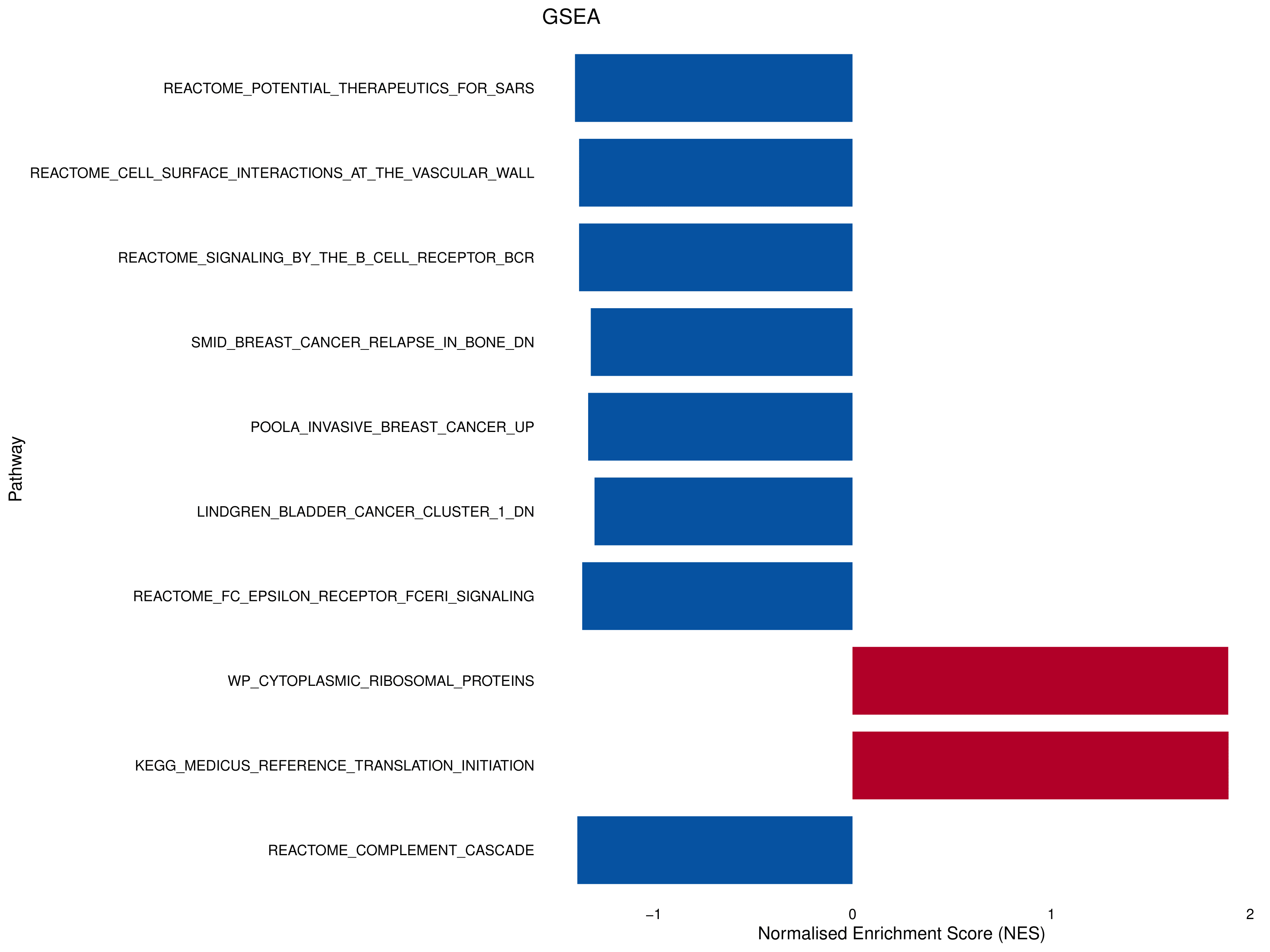
A quick note on where these gene sets come from. These are submitted by the academic community as "signatures" of particular experimental set ups. This means a gene set name may make absolutely no sense in the context of your work - such as "therapeutics for SARS" as the top hit in a bladder cancer comparison. But, think what this actually means - this is (likely) a set of genes involved in immune response. The interpretation here is that FGFR3 wildtype tumours have a better immune response. This matches the literature as active FGF signalling (most mutations in FGFR3 are activating) causes immune cell exclusion.
To explore these results, you can look at the leadingEdge column (these are the most significant hits from each gene set) and google the exact name of the pathway followed by "MSigDB" and you will find a webpage giving information on the paper/experiment used to create the gene list.
What now?
Excellent! Well done for getting to the end! This should be a page you keep coming back to during your project. Don't worry if you haven't understood it all - you'll be amazed how far you come this year. I'm looking forward to working with you and seeing what you find!